

In this blog post, we will continue our Hypothesis testing example and will be Calculating hypothesis test statistics.
Lets actually work with some numbers!
From our 3 previous blog posts:
- Creating a Hypothesis For Sample Testing
- Deciding the Correct Hypothesis
- Sample testing in China- hypothesis rules
We have the following:
- Null hypothesis, H0= All bags of crisps weigh > 32.51g
- Alternative hypothesis, H1 = Some bags of crisps weigh ≤ 32.51g
and…
- Alpha of 0.02
- A lower-tailed test decision rule
We almost have all the data around us to start to calculate our tests statistics.
We need to go back to our original question on the specifics of the test.
10,000 bags of crisps
We had a large population of 10,000 bags of crisps. We know that we can not weigh individually each bag of crisps.
So we want to get to a point where we can understand if we have a potential where any of of our bags of crisps could be underweight.
Let’s work out how we do that: We would probably split our 10,000 into a more manageable number. But even so, as long as we have the possibility to weigh the mean it doesn’t really matter as long as we have the mean value and standard deviation we can get confidence in our stats.
So for example sake: We have a batch of 500 (out of our 10,000).
N number
That’s the first number we need; we name this value the n number:
- n=500
The second is our standard deviation, we discussed about standard deviation in our blog post here: The Importance of sample size
Standard Deviation
Our standard deviation from the production of these crisps is:
- 1.6
Mean
The third number is the mean weight of our n. Here is where it gets interesting.
The mean of this 500 is 34.5g. We also spoke about the mean in our previous blog post: The Z score and How We Can Use it in Acceptance Sampling
So you would say, hey, wait, our mean average is 34.5g, that’s above our minimum 32.51g that we are using as our go/ no go cut off point? Surely we can let this batch go?
Wait, our original threshold was to ensure that no bags of crisps were released from factory below 32.51g.
The following calculation will give us the indication if we do in fact have this condition.
Z-Score
The first thing we want to work out is our Z score.
We spoke about the z score here: The Z score and How We Can Use it in Acceptance Sampling
Remember this calculation:
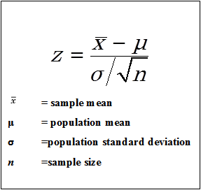
See how we have added the n number into the above equation. This is because we get the SD from the main population of data (our 10,000 crisps, yet we are doing a sample Z test on just 500 of these units). So we want to ensure that this data set is taking into consideration both the population of data and the sample set of data.
After plugging all the gaps in the above, it gets very complicated.
So I usually turn to Mini-Tab. But you can also write it out like this:
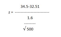
If we put the above numbers into the equation we come out with a Z value of 27.81. By the way, 27 is a massive number…
We then look at our Z table to convert this number to our P score. We talked about the Z table here: The Z score and How We Can Use it in Acceptance Sampling
Result
As it’s off the table we have a P-value of 0.
A 0 P-value is of course low.
If the P is low, we reject the null hypothesis:
- alpha = 0.02
- P-Value = 0
- a > P-Value = Reject Null Hypothesis
- 0.02 > 0 = Reject H0
Which means that we can state with 98% confidence in our batch of 500 we will have conditions where we have bags of crisps under our threshold of 32.51g meaning we have to reject this batch of crisps.
The null hypothesis, H0= All bags of crisps weigh > 32.51g- The alternative hypothesis, H1 = Some bags of crisps weigh ≤ 32.51g
In a real-world situation, you would have to go back to production and tighten up the production capabilities to reduce the variation. This, in turn, reduces the standard deviation.
Allowing you to ensure that you get more centralised standard production, less stock rejection and ultimately a better more refined product.
Conclusion:
You can now see that predicting the future does not have to be a Mystic Meg situation. You can tell, from a much smaller sample size on how to accept or reject batches of stock and the reasons behind why we do what we do.
This, of course, is what Lean and Six Sigma is all about. It’s about reducing your variation in manufacturing to give you a better product, a tighter production capability and an increase in profits.
This is a great example of the cost of poor quality.
We will be talking about why in another blog post. We will also be discussing how we can conduct hypothesis testing on much lower samples where we don’t necessarily have the standard deviation in front of us.
This is called single sampling T-tests.
I said before in a previous example of some statistical geekiness not to worry too much about understanding all this information in its entirety. Some great software tools do all the above calculations quickly. Even Microsoft Excel can do these calculations.
If you want any advice on sample testing, or indeed you want us to have a look at any of your samples please get in touch here, or connect with us on LinkedIn here and follow Merchsprout here.