

The Z Score And How We Can Use It In Acceptance Sampling
In our last blog post, we talked about how Standard deviation can allow us to understand if data points are away from the mean and by how much. In this post, we are going to discuss how we can calculate the Z score and how we can use it in acceptance sampling.
The Z score
The Z Score… Sounds like some 80’s throwback TV series.
But in reality, if we want to use Six Sigma in our sampling analysis it’s a number that we need to understand.
In our previous blog, we spoke about how a bell curve can allow us to understand how data is arranged, and how many points away from the mean data should fall if we want to conform to Six Sigma process.
The Z score is the score of an individual data point away from the mean, expressed in standard deviation.
As we know 99.7% of data points should fall within 3 sigma +/- of the mean. We can, therefore, use the Z score to determine if we have a potential error state in any given samples.
This is also known as Empirical rule.
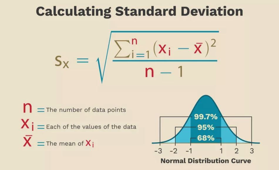
The Calculation
Z= Z score
x=observed value
x (bar) =mean of the samples
s=standard deviation of the samples
For our Z score to make any sense, first of all, we need to work out a few things.
The first being our standard deviation.
I am going to cheat somewhat and use a program called MiniTab.
You can have a look at Minitab on Google. It’s an amazing piece of software with endless possibilities, I have a good friend who used to spend all of his ex-pat years using probability software to try and predict horseracing.
He would come into work in the morning with bags under his eyes, I don’t know if he ever cracked it.
But I had good fun at his expense.
I digress, but if you like statistics be sure to check it out.
Random Data
To work out standard deviation on normalised data we can input data into Minitab (much the same as an Excel file):
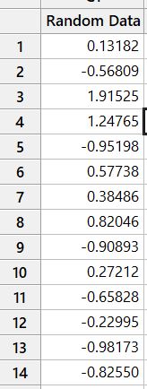
This is a selection of random normalised data ranging from a value of -3.0649 to 2.6768.
It has 150 data sets.
Don’t get too hung up on the range of values.
If it makes it any easier: imagine the data as a dimension on a cylinder being measured at the end of the line.
Or a range of temperatures in the Siberian wilderness through September…
I don’t know… Use your imagination.
Either way, we have 150 random data points that are normalised.
We can now work out from these data sets the standard deviation using the standard deviation calculation.
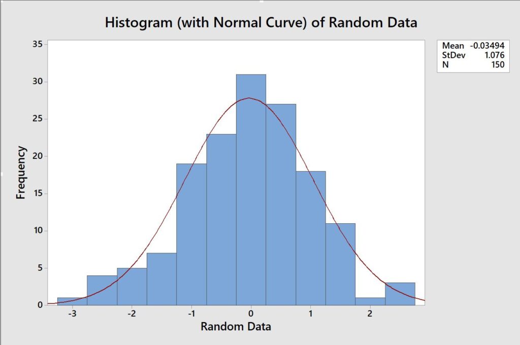
Our histogram from random data
So now I bet you are like yeah… so what, what does this even mean to me?
Well, let’s revisit our Z score and determine if a single value conforms to our empirical rule that 99.7% of data should fall within 3 standard deviation points.
We can see that we have all the data around us now to work out the Z score.
We have the Mean of our data at -0.03494.
Our standard deviation of 1.076.
All we need to work out our Z score is our single data set.
And we can do that here:
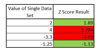
You can see from the above data you can start to draw a picture to determine if a given value is within the limit allowed for six sigma standard deviation.
2 of the above scores are over the limit of our 3 standard deviations.
If we were basing hypothesis’ off this data we would have to look at error states and potentially reject.
Well, kind of…
We will be going into hypothesis testing in a later blog post.
The importance of understanding the Standard deviation and Z scores is important when calculating hypothesis, and general sample testing working to Six Sigma.
Z Score Tables
Because we know that 68% of data fall within +/- 1 SD of the mean, 95% within +/- 2 SD of the mean and 99.7% of data within +/- 3 SD of the mean, we can use the Z number, and Z table to work out precisely how many data points are either side of the Z score; as a percentage.
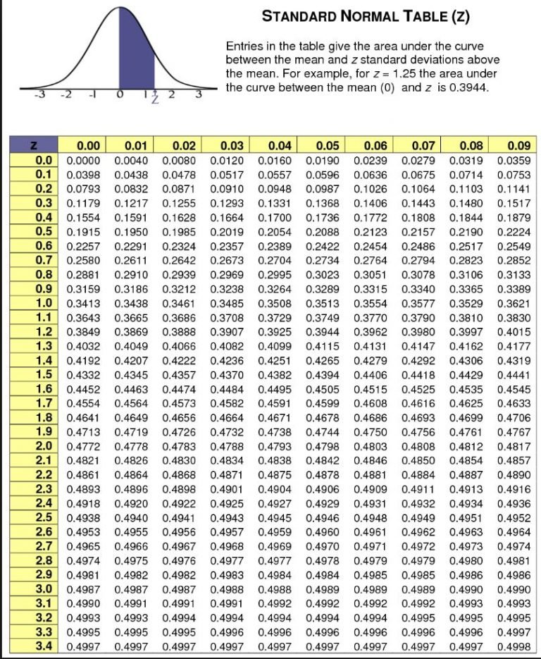
We use the standard normal table (Z) above by corresponding our Z number:
Our single value of 2 had a Z score of 1.89, meaning that the score of 2 was within a + gap of 1.89 standard deviations from the mean.
We can then look at the table above and can see that if we go to 1.89 we get a value of 0.4706, we then times this by 2, giving us a value of 0.9412, meaning that 94.12% of the data is to the left of this point in our normalised bell curve table.
We use this number in a later chapter when we look at Hypothesis testing.
Conclusion
Don’t worry too much if some of this went deep into statistical analysis.
When we conduct sample analysis to six sigma we don’t have to delve this deep into the data.
But it is really useful to understand why we are given the numbers that we are.
We use Minitab the majority of the time to highlight sample thresholds and if sample batches can be accepted or rejected.
In future blog posts, we explain some real-life examples of how we apply these techniques; and have either signed off or rejected components based on acceptance levels based on batch and sample size.
If you want any advise on sample testing, or indeed want to discuss with us how you can have the quality of your components checked by our team of experts in China. Contact us, leave a comment or add us on Linked In.